|
Navigation: Toolboxes > Control Toolbox > Controller Design Editor > State Space Models |
  
|
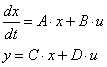
State space models use linear differential equations (continuous) or difference equations (discrete) to describe system dynamics. They are of the form:
|
|
(continuous) |
(discrete) |
with for example:
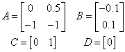
where x is the state vector and u and y are the input and output vectors. These models may arise from the equation of physics, from state space identification or as the result of linearization.
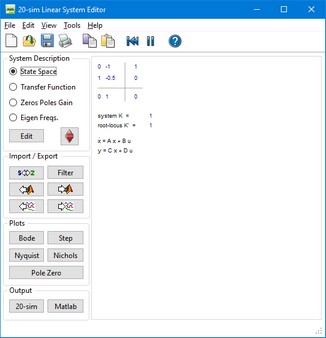
You can enter state space models by selecting the State Space button and clicking the Edit button.
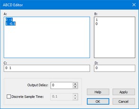
This opens an editor in which you can enter the A, B, C and D matrices. Depending on the selection of the Discrete Linear System check box (and Sample Time) the system is a continuous-time or discrete-time system. You can enter the matrix elements in the white space areas. Separate column elements with Spaces or Commas. Enter new rows by clicking the Enter key (new line) or using a semicolon. Brackets ( e.g. [ ... ] ) may be used to denote the a matrix or vector.
The A-matrix, shown in the figure above can for example be entered as:
0 1
-0.5 -1
or
0,1;-0.5,-1
or
[0,1;
-0.5,-1]
To inspect the effects of time delay in your model, you can add output delay. The result will be visible in the various plots that you can show of a linear system. The unit of the output delay is seconds.
If you want to transfer a linear system from continuous time to discrete time directly (i.e. replace the s by a z), select Discrete Sample time and fill in the sample time value. You can also transfer back directly by deselecting Discrete Sample time.
| • | Help: Open the help file. |
| • | Apply: Apply the current changes of the system, recalculate each plot that is active (step, Bode, Nyquist, Nichols, pole zero). |
| • | OK: Apply the current changes of the system, recalculate each plot that is active (step, Bode, Nyquist, Nichols, pole zero) and close the editor. |
| • | Cancel: Do not apply any changes to the system and close the editor. |