


Static and Dynamic Phenomena |
  
|
The friction phenomena can be grouped in static and dynamic phenomena:
| • | static friction phenomena: |
| • | static friction |
| • | Coulomb friction (dynamic friction) |
| • | viscous friction |
| • | Stribeck friction (Stribeck effect) |
| • | dynamic friction phenomena: |
| • | pre-sliding displacement (Dahl effect) |
| • | rising static friction (varying break-away force) |
| • | frictional lag |
Static friction models only have a static dependency on velocity. Even when the applied force is very small, the result is a non-zero velocity. This means a significant displacement is found after some time. Therefore static friction models should only be used in systems where the applied forces are large (>> static friction), or change sign often.
Dynamic friction models incorporate a spring like behavior for small forces. I.e. no significant displacement is found when the applied force is smaller that the static friction.
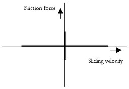
Static friction phenomena only have a static dependency on velocity. The first static friction model was the classic model of friction of Leonardo Da Vinci: friction force is proportional to load, opposes the direction of motion and is independent of contact area. Coulomb (1785) further developed this model and the friction phenomena described by the model became known as Coulomb friction. The model is given in the figure below.

The Coulomb friction model.
The friction force can be described as:
Ff = Fn * mu_c * sign (v);
with mu_c the Coulomb friction coefficient. The Coulomb friction model is, because of its simplicity, often used. In many textbooks is is also referred to as dynamic friction and mu_s described as the dynamic friction coefficient.
Morin (1833) introduced the idea of static friction: friction force opposes the direction of motion when the sliding velocity is zero.
The static friction force is equal to the tensile forces until a maximum or minimum is reached:
Ff_max = Fn * mu_s;
Ff_min = -Fn * mu_s;
with mu_s the static friction coefficient.
Reynolds (1866) developed expressions for the friction force caused by the viscosity of lubricants. The term viscous friction is used for this friction phenomenon.
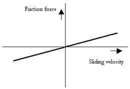
The viscous friction model.
The friction force can be described as:
Ff = Fn * mu_v * v;
with mu_v the viscous friction coefficient.
This viscous friction combined with the Coulomb friction gave the model given in the figure below.

The Coulomb plus viscous friction model.
When static friction is added, a friction model appears that is commonly used in engineering: the Static plus Coulomb plus Viscous friction model. This model is depicted in the figure below.

The static, Coulomb plus viscous friction model.
Stribeck (1902) observed that for low velocities, the friction force is decreasing continuously with increasing velocities and not in a discontinuous matter as described above. This phenomenon of a decreasing friction at low, increasing velocities is called the Stribeck friction or effect. The model including Static, Coulomb, Viscous and Stribeck friction is given below.

The static, Coulomb, viscous plus Stribeck friction model.
The Stribeck effect is described by the parameter v_st which is the characteristic Stribeck velocity. It denotes the sliding velocity where only a 37% of the static friction is active. In other words, small values of v_st give a fast decreasing Stribeck effect and large values of v_st give a slow decreasing Stribeck effect.
All these friction models above show a discontinuity at zero velocity. At zero velocity the friction force as a function of only velocity is not specified. What for example should the friction force be at zero velocity in the Coulomb friction model? The discontinuous behavior of this model near zero velocity is sometimes approximated with a continuous function, for example:
F = tanh(slope*v);
and the inverse
v = arctanh(F)/slope;
with slope a very large constant. The use of continuous functions results in straightforward models that are easy to simulate for large forces and velocities. For small forces and velocities, the the slope parameter has to be chosen sufficiently high, to avoid creep (the model starts to move, even when the applied force is smaller than the static or Coulomb friction force). This results in stiff models, which are hard to simulate.
The LuGre model is inspired by the bristle interpretation of friction (surfaces are very irregular at the microscopic level and two surfaces make contact at a number of asperities, which can be thought of as elastic bristles), in combination with lubricant effects.
Friction is modeled as the average deflection force of elastic springs. When a tangential force is applied the bristles will deflect. If the deflection is sufficiently large, the bristles start to slip. The average defection at steady state slip is determined by the velocity, so that for low velocities the steady state deflection, and therefore the friction force, decreases with increasing velocity. This corresponds to more lubricant being forced into the interface, and pushing the surfaces apart, as the velocity increases. This produces the Stribeck effect. The model also includes rate dependent friction phenomena such as varying break-away force and frictional lag. The model behaves like a well damped spring with a stiffness at zero speed for small motions.